BLUNDER LOCATION
Larry Fish
In 1979 I started working on
a project to computerize the survey data for Groaning Cave. The cave had been
discovered in 1969 and I was suddenly handed ten years of survey data that had
never been processed by a computer. The early surveyors had processed all the
information by hand and as a result, there many anomalies and problems in the
data.
When I looked at the Groaning
data, I found that many loops near the front of the cave had large loop closure
errors. Luckily, I had more than one survey for some of the worst loops and was
able to compare good surveys to bad surveys of the same passage. Much to my
surprise, the errors in the surveys were not due to the accumulation of small,
random errors; but were due to major blunders like reading the wrong end of the
compass needle, transposing digits on the survey notes, mixing up azimuth and
elevation, etc. By comparing good surveys to bad, I could easily fix a bad
survey by repairing the worst blunders one by one until the survey closed.
As I played with the idea
more, I discovered that I didn't always need a good survey to find the blunders
in a bad survey. I could see that each blunder leaves its own special mark on
the closure error. For example, an azimuth error has no effect on the vertical
component of the closure error, so a compass error can never produce a vertical
error. If you have a survey with one blunder in it, the blunder will produce a
very specific kind of closure error. For example, let say you have a 10 foot
length blunder on a shot that has an azimuth of 130 degrees and inclination of
-10 degrees, the closure error will be 10 feet on an azimuth of 130 degrees and
an inclination of of -10 degrees. To find the blunder, all you have to do is
find a shot that matches that measurement.
You can of course try to find
matches by hand, but this is very tedious. In addition, matching azimuth and
inclination is much more complicated. It is much more useful to locate the
errors using a computer. As a result, the COMPASS cave survey software has
special routines that can locate blunders in survey loops.
UNDERSTANDING SURVEY
ERRORS
In order to understand the
process of locating blunders, it is useful to understand something about survey
errors. There are three kinds of
errors that occur in a cave survey:
1. Random Errors.
2. Systematic Errors.
3. Gross Errors or
Blunders.
1. Random Errors. Random errors are generally small errors that occur
during the process of surveying. They result from the fact that it is
impossible to get absolutely perfect measurements each time you read a compass,
inclinometer or tape measure. For example, your hand may shake as you read the
compass, the air temperature may affect the length of the tape, and you may not
aim the inclinometer precisely at the target. There are literally hundreds of
small variations that can affect your measurements. In addition, the
instruments themselves have limitations as to how accurately they can be read.
For example, most compasses don't have line markings smaller than .5 degrees.
This means that the actual angle may be 123.4 degrees, but it gets written down
as 123.5.
All these effects add up to a
small random variation in measurement of survey shots. Even though these errors
are random, they tend to follow a pattern. The pattern is called a ”normal“
distribution and it has the familiar ”bell“ shaped curve. As a result of this
pattern, we can predict how much error there should be in a survey loop if the
errors are the result of small random differences in the measurements. If a
survey exceeds the predicted level of error, then the survey must have another,
more profound kind of error.
2. Systematic Errors. Systematic errors occur when something causes a
constant and consistent error throughout the survey. Some examples of
systematic error are: the tape has stretched and is 2 cm too long, the compass
has five degree clockwise bias, or the surveyor read percent grade instead of
degrees from the inclinometer. The key to systematic errors is that they are
constant and consistent. If you understand what has caused the systematic
error, you can remove it from each shot with simple math. For example, if the
compass has a five degree clockwise bias, you simply subtract five degrees from
each azimuth.
3. Blunders. Blunders are fundamental errors in surveying process.
Blunders are usually caused by human errors. Blunders are mistakes in the
processing of taking, reading, transcribing or recording survey data. Some
typical blunders are: reading the wrong end of the compass needle, transposing
digits written in the survey book, or tying a survey into the wrong station.
Blunders are the most
difficult errors to deal with because they are inconsistent. For example, if
you read the wrong end of the compass needle, the reading will be off by 180
degrees. If you transpose the ones and tens digits on tape measure, the reading
could be off by anything from 0 to 90 feet.
THE ACCUMULATION OF SURVEY
ERRORS
As you survey around a loop,
the errors slowly accumulate, which effects how well the loop closes. It is
important to understand how survey errors accumulate, because it allows us to
make predictions about how well each loop should close. If you know how a loop
should close, you can assess the quality of the survey measurements and the
accuracy of the map as a whole.
Let's look at the way errors
accumulate as you survey a cave. Let's say that you have a series ten foot
shots and you have a ruler that is only accurate to plus or minus one foot.
That means that sometimes you will read nine feet, sometimes ten feet and
sometimes eleven feet and sometimes in between. As a simple example, here are
the results of three length measurements:
Result: A B C
Measurement: 9 10 11
Error: -1 0 +1
Notice that the error is
minus one, zero and plus one.
If you combine the errors from
two shots something very interesting happens. First since there are three
results for each shots, there are a total of nine combinations:
A + A'
= -1 + -1 = -2
A + B'
= -1 + 0 = -1
A + C'
= -1 + +1 = 0
B + A'
= 0 + -1 = -1
B + B'
= 0 + 0 = 0
B + C'
= 0 + +1 = 1
C + A'
= 1 + -1 = 0
C + B'
= 1 + 0 = 1
C + C'
= 1 + +1 = 2
As we add together all the
possible errors from two shots, the error begins to spread out. The lowest
combined error is -2 and the highest combined error is +2. If we count how many
shots fall into each error total, we get the following chart:
-2 -1 0
-1 0 +1
0 +1 +2
-------------------
Total In Each
Range: 1 2 3 2 1
Notice how the results tend
to concentrate in the middle and thin out toward the edge. If you combine
enough shots in this way, then we will get the familiar ”bell shaped“ curve.
This also gives us the probability of various total errors at the end of a
three shots.
1 chance
in 9 the error will be -2.
2 chances
in 9 the error will be -1.
3 chances
in 9 the error will be 0.
2 chances
in 9 the error will be +1.
1 chances
in 9 the error will be +2.
This kind of information is
very useful for determining the quality of a loop. For example if you get a
loop error of minus three for the example survey, the chances are less than one
in nine that it is a random error. Thus, it is very useful to be able to
predict the kind of errors you should find in a loop.
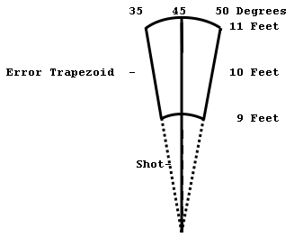
TWO DIMENSIONS
So far, we have only looked
at errors in one dimension. If we added in the error caused by the compass
reading, the error becomes two dimensional. For example, lets say that you have
a ten foot shot and 45 degree compass bearing. Lets also say that length is
accurate to plus or minus one foot and the compass is accurate to plus or minus
ten degrees. This will produce an error pattern that looks something like a
rounded trapezoid:
If we combine the errors
trapezoids for two shots the way we did in the first example, the two
trapezoids will add and overlap. As before, most of the combinations will
cluster in the middle and thin out toward the edge. This forms a kind of three
dimensional bell shaped curve.
Another thing that happens
with errors from two measurements is the values vary depending on the angle of
the shot. For example, lets say that we have a shot with a compass angle of
zero. If there is any uncertainty in the angle, then we will get errors in the
east/west direction. Likewise, if the compass angle is 90, then errors will be
in the north/south direction. Finally, if the shot is at 45 degrees, the errors
will be equally north/south and east/west. As a result, we have to take into account
the angle of each and every shot, before we can make a prediction about the
loop error.
THREE DIMENSIONS
The same principles that we
have used for two measurements apply to three. Using compass, length and
inclination makes the potential errors cluster in a sort of spherical shape,
and most of the results will concentrate around the center.
LOCATING BAD LOOPS.
Since we know the kind of
pattern that random errors produce, we should be able to detect those
situations where the errors more than random. In other words, we should be able
to single out those loops that have errors that are likely caused by blunders.
To do this, we need to make a prediction about the size of error we expect to
see. If the actual error is greater than this amount, then the loop probably
has a blunder in it.
To make a prediction about
the size of error we expect, we need to know how accurately each instrument can
be read. For example, if you can read a compass accurately to within one
degree, every azimuth reading will have an ”uncertainty“ (or ”variance“) of
about one degree. Each type and brand of compass, tape measure and inclinometer
has a different level of ”uncertainty“ associated with it. For example,
experiments on a test survey courses show that Suuntos are more accurate than
Sustecos and Sustecos are more accurate than Silvas. Also, some surveyors are
better than others and some caves are more difficult than others. All this adds
up to varying levels of uncertainty in the survey measurements.
If you combine all these
uncertainties around the loop, you will get a prediction of what the total
error should be if all the errors are random. Notice, that each shot has a
different effect on the outcome. For example, if the shot is heading north, a
one degree azimuth uncertainty adds to the east/west errors. If the shot is
heading east, the uncertainty adds to north/south errors. If you have loop with
more shots in the north/south direction, you would expect the loop to have more
east/west error. For this reason, every measurement in every shot should be
used to make a prediction of the error.
The resulting prediction is
the ”standard deviation“ for the loop. Since the errors in a loop should be
random (unless there is a blunder or systematic error), standard deviation is a
good way to predict whether the loop has a blunder. The best way to understand
standard deviation is to look at a graph:
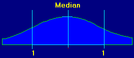
This
is a graph of a typical set of random events. Again, this is the famous ”bell shaped“ curve. It gives a
visual representation of how the events are distributed. The events could be
things like rain fall in Florida, wins on a roulette wheel or cave survey
measurements. The center of graph is called the median and it is the average of
all the events. You will notice that like our survey errors most of the events
fall into the middle of the graph. Also, as you move to either edge, there are
fewer events. At the bottom the graph, standard deviations are marked. They are
numbered going away from the center. This is because we care about how far a
particular measurement is from the average.
Standard deviations are a
measure of how much variability there is in the data. The more variability, the
larger the standard deviation will be. If you look at the second graph above,
Here is another graph:
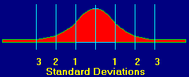
You will notice that the data
is more tightly clustered around the center. This means that the data has less
variability. You can see that the standard deviations are smaller. If this were
cave data, the tight clustering would mean that the cave was surveyed more
carefully or with better instruments.
When we are looking for loops
with blunders, we look for loops whose errors fall on the edge of the bell
shaped curve. For example if we have a loop whose error falls ”three standard
deviations from the mean,“ we would be very suspicious that the loop had a
blunder. In other words, the standard deviation for a loop gives you a range of
values that can be expected if the errors are random.
LARGE ERRORS AREN'T ALWAYS
BLUNDERS
Another important aspect of
random errors is that over the course of a loop, the errors tend to cancel each
other out. For example, sometimes you will read the compass half a degree
positive, sometimes half a degree negative and sometimes right on. If you add
up all these positives and negatives, the resulting error will be relatively
small.
There is however, a small
chance that the errors will fall in such a way that there will be a larger
error. Sometimes, by random chance, most your compass readings will end up half
a degree negative. This will give you a larger error even though there is no
real blunder. It's like flipping a coin. Most of the time, you expect 50% head
and 50% tails, but every once in a while, you will get five straight tails in a
row. If you get five straight compass readings that are half a degree low, the
error will be disproportional large.
So another way of
understanding errors is to look at them as odds and chances. As the standard
deviation goes up, the odds of the loop being blundered goes up. For example,
if the standard deviation is 2, there is 5 chances in 100 that it is not a
blunder. But if the error is 3 standard deviations, there are only 3 chances in
1000 that it is not a blunder.
The chart below gives more
exact numbers for various standard deviations.
Standard
Deviation Percent Inside Percent Outside
0.5 38.30 % 61.70 %
1.0 68.26 % 31.74 %
1.5 86.64 % 13.36 %
2.0 95.44 % 4.56 %
2.5 98.76 % 1.24 %
3.0 99.74 % 0.26 %
You can see that if you have
a loop with no blunders and only random errors, the loop error should fall
within one standard deviation 68 percent of the time. By looking at the number
of standard deviations a loop is away from our predicted error value, we get a
clear idea about the quality of the loop. In simple terms, here is what the
numbers mean:
BETWEEN 0 AND 1: If the value
is between 0 and 1 the loop is of very high quality and probably does not have
any blunders or systematic errors.
BETWEEN 1 AND 2: If the value
is between 1 and 2, the loop is still probably good, but there is a greater
chance the errors are caused by blunders.
GREATER THAN 2: If the value
is greater than 2, there is a high probability that the loop has a systematic
error or a blunder.
You can also make some
inferences about the kind of blunder you have by looking at the size of the
error:
Small Errors. 1 - 5 Standard
Deviations.
Errors
between one to five standard deviations generally are seen when there is a
misreading of the instruments. For example, you could get this type of reading
if you misinterpreted an azimuth of 320 as 330.
Medium Errors. 3 - 20
Standard Deviations.
Errors
between three to twenty are seen with shot reversal. For example, if you read
the wrong end of the compass needle or do a back sight without reversing the
stations. This would give a reading that is incorrect by 180 degrees. The size
of the errors is governed by the length of the shot. Long shots produce bigger
errors.
Large Errors. 15 - 100
Standard Deviations.
Errors
greater than fifteen standard deviations are seen in situation where a survey
has been tied into the incorrect the incorrect station. For example, if a
survey is supposed to connect to station B12 and instead is connected B13, a
large error will probably result. The size of the error will depend on how far
the erroneous station is from the correct station.
These numbers are very
general rules of thumb. Actual error can vary depending on the exact
circumstances. For example, if you have a shot reversal on a very short shot,
the error could easily be less than one standard deviation.
LOCATING INDIVIDUAL
BLUNDERS.
The whole point of looking at
the standard deviations of loops is to find loops that probably have blunders
in them. After you have located loops with large deviations, the next step is
to analyze the loop looking for the specific measurement that has caused the
blunder.
The basic concept of blunder
location is fairly simple: If you have a blunder and you fix it, the loop error
should go down significantly. Thus, the trick to finding blunders is to find a
measurement that when adjusted, makes the loop error go down significantly. The
way to do this is to go around the loop adjusting each measurement, one at a
time, trying to get the most improvement for that particular measurement. The
adjustment that makes the biggest improvement in the loop error is the most
likely candidate to be the blunder for that loop.
Since you adjust each
measurement one at a time, the adjustment is constrained by the other
measurements in the shot. As a result, there is a limit to how much improvement
each adjustment can produce. For example, if you test-adjust the azimuth of a
10 foot shot, the result must fall on a circle with a 10 foot radius. This
constrains the possible improvement to the circle. If the measurement is not
the blunder, it very unlikely that the adjustment will significantly improve
the loop error. This means that blunders leave unique signatures on the loop
error.
By going through the survey
and adjusting each measurement in turn, you will find that most adjustments
make only modest improvements in the loop error. However, if you adjust the
blundered measurement, it will produce a dramatic improvement in the loop error.
In other words, the best adjustments will always correspond with the worst
blunders.
BLUNDER SIGNATURES
Another way of looking at
blunders is that they leave a signature on the error value. For example, lets say
that you have made a blunder on a length measurement so that the shot is ten
feet too long. This will add ten feet to the loop error. More important, the
ten foot error will be in a direction that matches the azimuth and inclination
of the shot. If the shot had an inclination of 10 degrees and an azimuth of
173, the error would be 10 feet in the direction of 173 azimuth, 10 degrees
inclination. This creates a blunder signature that is unique. This means that
only shots with same azimuth and inclination could cause the error that we see.
As a result, it is often possible to zero in on the exact measurement that
caused the blunder.
The signatures are often
unique because there are two measurements that leave their mark on the
signature. In our example, the combination of azimuth and inclination controls
the signature. The odds of having these two measurements match exactly in a different
shot are fairly low.
Even when you have an error
signature that matches two or more shots, all is not lost. When two or more
shots produce a signature that matches the error, you cannot be sure which shot
has caused the error. However, you still have narrowed the number of likely
candidates.
Again, the actual process of
locating blunders is done by examining each and every measurement looking to
see if it matches the error signature. You save the most successful
adjustments. Since these are adjustments that do the best job of fixing the
error, they are most likely candidates for blunders.
BLUNDER SENSITIVITY
There are several things that
effect how well you can find blunders.
1. Loop Quality. Blunder
location works best where the quality of the rest of the loop is high. If the
unblundered shots in a loop have a high random error level, the blunders become
overwhelmed by the accumulated random errors around the loop. The following table
shows the sensitivity level vs. error level:
Unblundered
Length Azimuth Inclination
Error Level
Sensitivity Sensitivity Sensitivity
0 - .3 STD
1 Foot 1 Degree 1 Degree
.3 - 1 STD
5 Feet 5 Degrees 5 Degrees
> 1
STD >10 Feet >10 Degrees >10 Degrees
2. Large Blunders vs Small
Blunders. Large blunders are usually easier to detect than small ones. However,
this can be tricky. For example, a 180 degree error may seem large, but if it
is on .5 foot shot, the resulting error is less than a foot.
3. Multiple Blunders. If you
have two or more blunders in a loop, each individual is more difficult to
isolate. Two blunders on the same shot are almost impossible to isolate. If
there are two blunders on different shots, one blunder tends to dominate and
obscure the other.
4. Unique Signatures. The
more unique the blunder is, the more likely it will be isolated. For example,
lets say you have a blunder on a shot with a compass reading of 180 degrees. In
addition, lets say that there are no other shots that come to within 45 degrees
of the blunder. This blunder will be so unique that it can be isolated even in
a relatively low quality loop. On the other hand, if you have many shots with a
similar azimuth, random errors in the rest of the loop can cause the program to
select several shot as the possible blunder shot. If you see several candidates
with the similar ”Change“ values and similar improvement ratios, it may
indicate that the blunder is not unique enough to be isolated. You can however,
narrow it down to a few candidates.
5. Blunder location works
slightly better on small loops. As the loop grows longer, random errors make a
larger contribution to the error. Eventually, the accumulation of random errors
becomes large enough so that the effect of the blunder is lost.
INTERSECTS
Once you have a list of good
blunder candidates, there is another technique you can use to narrow your
choices. The technique is called”Intersects.“ If a blundered shot participates
in two loops, it should have a similar blunder signature in both loops. If it
doesn't, you can pretty much eliminate it as a blunder candidate. Likewise, if
the shot participates in more than two loops, it should have a similar blunder
signature in all the loops. The only exception is the case where one of the
other loops has an additional blunder which masks the original blunder. Even
so, a blunder should show up with the same signature in most of the loops. This
technique is very useful because it can eliminate candidates and narrow the
field to just a few shots.
To give you an idea how
intersects work, I have included some actual cave data from Lechuguilla cave
showing two potentially blundered shots.
From To
Measure Change New Error New Dev. Improvement
EPB1 GZ1
Length 21.49 Ft. 3.95 0.91 5.54
EPB1 GZ1
Length 20.36 Ft. 4.29 1.04 4.85
EPB1 GZ1
Length 24.34 Ft. 5.57 1.05 4.48
EPB1 GZ1
Length 24.40 Ft. 6.70 1.25 3.78
EPB1 GZ1
Length 23.18 Ft. 6.68 1.21 3.61
EPB1 GZ1
Length 21.85 Ft. 7.80 1.55 2.98
GZ4 GZ5
Azimuth -68.91 Deg 1.99 0.46 10.98
GZ4 GZ5
Azimuth -67.01 Deg 2.51 0.61 8.28
GZ4 GZ5
Azimuth -77.08 Deg 3.24 0.61 7.71
GZ4 GZ5
Azimuth -76.00 Deg 4.36 0.79 5.54
GZ4 GZ5
Azimuth -77.80 Deg 4.64 0.87 5.45
Notice that the first shot
participated in different six loops, the second shot participated in five different
loops. Also, notice that the ”change“ value is remarkably consistent between
all the different loops. This means that the we are finding the same signature
in completely different loops. This is highly indicative that the shot is a
blunder.
BAD TIE-INS
One of the most common types
of blunders occur when a shot is tied to the wrong station. This can happen
through typos, misplaced stations in the cave and renaming stations after the
survey is complete. Connecting a shot to the wrong station can cause very large
survey errors.
It is possible to locate bad
tie-ins, by breaking a loop at one of the stations in the loop. This allows the
point at the break to move to its natural location. If there is bad tie-in,
this point will move back toward the proper station. If the loop was incorrectly
tied at the location of the break, the distance between the broken shot and the
correct tie-in will be near zero. Thus the process for locating a bad tie-ins is
to break the loop at every station around the loop and then keep track the
closest connections.
With a list of the best
candidates for bad tie-ins, the obvious typographical errors are easy to see. For
example, here are some obvious examples of mis-ties in the Lechuguilla data set
that were located using the technique:
OLD TIE
NEW TIE OLD ERROR NEW ERROR
K6 K6! 174.64 ft.
6.19 ft.
ECKJ11 ECKJ'11 152.78 ft. 1.75 ft.
BNM4 DNM4 127.52 ft. 3.44 ft.
EY52a EY52A 87.47
ft. 5.39 ft.
As you can see, all of these
mis-ties are due to obvious topographical or clerical errors.
DIFFICULT CASES
The blunder indications are
not always as clear cut as the example described above. In many instances,
there will be several good candidates for blunders. This can make it difficult
to isolate the specific measurement that has caused the blunder. In these
situations, it helps to have more insight into the finding process. Here are
some of the most important issues:
1. Looks for loops that have
errors greater than one standard deviation.
2. Look for ”Changes“ that
cause high ratios of improvement.
3. Look for situations where
there are multiple changes to the same measurement with similar values. For
example, if you see four shots with 10 foot changes to the length, chances are
very good that there is a 10 foot error in one of those shots.
4. Look for situations where
most of the changes are to the same type of measurement. For example, if all
the changes are to the azimuth measurement, then it is very likely that there
is a blunder in the azimuth.
5. Look for situations where
two or more loops share the same shot. If both loops indicate a blunder on the
same shot and measurement, chances are very good that a blunder exists in that
shot.
THE BLUNDER ALGORITHM
The actual technique for
locating blunder involves complicated three dimensional geometry. If you are
not mathematically inclined, you may want to skip this section.
The actual blunder location process
consists of two steps: 1. Locating blundered loops. 2. Locating blundered
measurements.
1. Locating Blundered Loops.
As stated above, the process
of locating blunders in survey loops involves making a predictions about the
size of error you should find if a loop contains random errors and no blunders.
The key is making the prediction.
The process of deriving the
prediction is fairly straight forward. Basically, the program starts with a
standard deviation for compass, tape, and inclination. The user can enter any
value he chooses for these values. The program then uses the standard deviation
for each instrument on each shot to calculate standard deviations for each shot
in the loop. All these deviations are combined to get a deviation for the whole
loop. This is the prediction.
It is important to apply the
standard deviations to each shot individually because each shot has a different
effect on the overall standard deviation. For example, if you have a loop with
lots of north-south shots, the standard deviation in the azimuth will produce
more east-west deviation.
The process of applying
standard deviations to each shot is fairly simple. With standard trig, you
calculate the Cartesian standard deviations for each shot. You then calculate
the sum of all the squares of the standard deviation. This is the variance for
the loop, and the square root of the variance is the standard deviation for the
loop.
In order to validate these
concepts, algorithms and routines, I wrote a simulation program. The program
works by building a simulated cave survey about 100 shots long. The azimuth,
length and inclination of each shot is randomly selected. The program then
traverses the survey repeatedly, generating random Gaussian distributed errors
for each measurement in each shot. Each random Gaussian distributed error is
scaled to match the standard deviations assumptions for each measure. At the
end of each traverse, the program calculates the resulting error. After
accumulating 100 error sets, I calculate the standard deviation of the errors.
The program also uses the techniques I described above to make predictions
about the same loop. This way, I can compare the predictions against the actual
standard deviations simulated loop. At least in this setting, the routines
accurately predict the standard deviations I find in the simulated loops.
2. Locating Blundered
Measurements.
Once you have located loops
that exceed the predicted error levels, you can zero in on the actual
measurement that has caused the blunder. The technique for zeroing in on
individual blunders involves finding an adjustment that makes the best
improvement for each measurement in a shot. The trick is to find simple
routines that calculate the best adjustments for azimuth, inclination and
length measurements. The following section describes the algorithms for finding
the best adjustment for each measurement.
AZIMUTH ADJUSTMENT
Figure 3 represents a closed
cave survey loop. Point S is the start of the survey, point E is the end of the
survey. The angle at A1 is the angle we are going to adjust. The object is to
find how much to change angle A1 to produce the best closure.
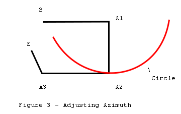
If we rotate angle A1 through
360 degrees, point A2 will describe a circle whose radius is equal to the
distance between point A1 and point A2. Since the azimuth angle measurements in
cave surveying are referenced to magnetic north, point A2 tends to be a hinge
point. That is, as A1 is rotated, the angle at A2 also changes but every angle
at every shot from A2 to the end of the survey stays the same. As a result, as
A1 is rotated, E describes a secondary circle whose center is offset from A1.
The secondary circle is
important because it represents all possible points that E can occupy as we
adjust angle A1. Thus, the best closure must be somewhere on it's
circumference.
In figure 4, C represents the
center of the secondary circle. This center C is located by taking the offset
between A2 and E and adding it to A1. To find the best closure, we must find
the point on the circle that is closest to the starting point S. Since the
shortest distance between any point and a circle must be on a radius, the best
closure must be at the point where the line C - S intersects the circle.
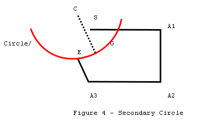
We know the locations of
S,E,A1,A2,C and the radius, so all of the remaining points and angles can be
calculated from this information.
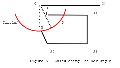
In figure 5, we construct a
horizontal line from C to H; and using point S, we construct a right triangle.
The location of G, the point of best closure, can be located using the triangle
and polar coordinates. The new closure error is the distance between G and S,
and the adjustment angle is the difference between angle G-C-H and angle E-C-H.
LENGTH ADJUSTMENT
Adjusting length is more
complicated because the shot length has both the azimuth angle and inclination
angle effecting it. As a result, the shot length is actually a vector in three
dimensional space.
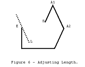
Adjusting a particular shot
for best closure is, in some ways, similar to adjusting azimuth. For example,
figure 6 represents a plan view of the survey, where S represents the start of
the survey and E the end of the survey. The survey has a large survey error. If
we attempt to minimize the closure error by adjusting the shot length of A1-A2,
point E will move, drawing line L which represents all possible adjustments of
the shot. Obviously, the best adjustment will give the shortest distance
between point S and line L.
Since we are working in three
dimensions, it is easiest to work using vector algebra. The shortest distance
between a point and a line in 3-D space is given by the following formula:
d=|U
x V|
In other words, the distance
from a line to a point is equal to the length of the cross product of the unit
vector U and vector V. In this case, V is the vector E-L and U is the unit
vector for line A1-A2. Since A1-A2 and E-L are parallel, we define E-L from
A1A2:
L=DXi
+ DYj +DZk
From this we find the unit
vector:
U = EL
/ |EL|
The distance is then
calculated using the cross products:
d=
|U x ES|
Once we have found d, we have
two sides of a right triangle and all other dimensions can be easily
calculated.
INCLINATION ADJUSTMENT
Adjusting the inclination
angle is the most difficult part of the closure process. Since it is an angular
adjustment, it is similar to the azimuth adjustment except that it takes place
in three dimensions. This is because the inclinometer is free to rotate around
the vertical axis, where as the compass is always held in the horizontal plane.
Figure 7 is a profile plot of
a survey. The vertical or Z axis is toward the top of the page. Point S
represents the start of the survey and point E represents the end of the
survey. As you can see, there is a closure error between S and E.
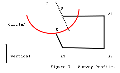
In this example, A1 will be
the inclination angle that will be adjusted. As with the azimuth adjustment,
when A1 is rotated through 360 degrees, A2 describes a circle with A1 as the
center. Since all of the shots from A2 to E remain unchanged, as the adjustment
is made, A2 will hinge and E will move through a secondary circle offset from
A1. Since the secondary circle represents the result of all possible
adjustments, the best closure must be some point on the secondary circle. The
task is to find the closest point on the circle to the starting point S. This
will be the best possible closure we can attain by adjusting the dip angle at
A1.
Since the secondary circle
and the starting point S are in three dimensions, the process of finding the
closest point is more complex.
Figure 8 represents a three
dimensional view of the secondary circle. Point S is the start of the survey
and point E is the end of the survey.
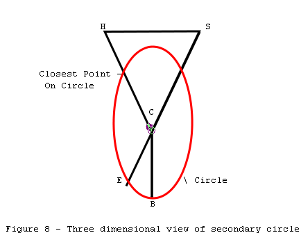
The strategy for finding the
closest point on the circle to S is to find the closest point from S to the
plane of the circle. In the diagram, H is the closest point in plane of the
circle to S. Now we calculate the intersect between H-C and the circle. This
will be the closest point to S and will represent the best possible adjustment
for this shot.
Since we know the location of
E and can calculate the location of B and C, this gives us two vectors in the
plane of the circle: C-B and C-E. By taking the cross product of CE and CB, we
get a vector perpendicular to the plane. Taking the dot product of C-S and the
unit vector of the perpendicular, we get the distance between S and the closest
point on the plane: point H. Adding a perpendicular vector of length H-S to the
coordinates for S gives us the coordinates for point H. With these coordinates,
all other coordinates, angles and distances can be calculated.
In order to clarify the
adjustment process, I have included the actual subroutines used in my blunder
detection programs. The code is written in Turbo Pascal.
The code sample consists of
three subroutines TESTAZM, TESTLEN and TESTINC which correspond with each
measurement in a shot. For example, ”TESTAZM“ finds the best adjustment for the
azimuth of a shot.
Each subroutine take four 3D
points as input. These four points are represented as 12 global variables which
give the cartesian coordinates of the points. The four points are:
1. The starting station of
the loop in: EAST0, NORTH0, VERT0; 2. The unclosed ending station of the loop
in: EAST9, NORTH9, VERT9 3. The starting station of the shot being tested:
EAST1, NORTH1, VERT1 4. The ending station of the shot being tested: EAST2,
NORTH2, VERT2
Each subroutine returns an
adjustment value for that particular measurement. The adjustment is stored in
the global variable ”ADJUST.“ The units of the adjustment depend on the type of
measurement. For example, ADJUST will return degrees from the azimuth ajusting
routine. The new error vector that results from each adjustment will be
returned in VECERR. The variable ”RC“ is used to convert between radians and
degrees.
Program Listing:
procedure  TESTAZM;
{ Test  The Azimuth Of A Specific Shot }
var
	NCENT,ECENT,	{ Circle Center }
	OPS,ADJ,HYP,	{ Sides Of Triangle }
	A,B,		{ Sides Of Triangle }
	RADIUS,		{ Radius Of Circle }
	PANGLE : double;		{ Polar Angle }
begin
{ Locate Center Of Circle }
NCENT:=NORTH1+(NORTH9-NORTH2);
ECENT:=EAST1+(EAST9-EAST2);

{ Calculate Radius }
A:=NORTH1-NORTH2;
B:=EAST1-EAST2;
RADIUS:=SQRT(SQR(A)+SQR(B));

{ Construct Triangle And Find Polar Angle }
OPS:=NORTH0-NCENT;
ADJ:=EAST0-ECENT;
HYP:=SQRT(SQR(OPS)+SQR(ADJ));
PANGLE:=ArcTan2(OPS,ADJ);

{ Calculate New Closure Error }
ADJ:=HYP-RADIUS;
OPS:=VERT9-VERT0;
VECERR:=SQRT(SQR(OPS)+SQR(ADJ));

{ Calculate Adjustment Angle }
OPS:=NORTH9-NCENT;
ADJ:=EAST9-ECENT;
ADJUST:=PANGLE-ArcTan2(OPS,ADJ);
ADJUST:=ADJUST*RC;
if ADJUST>180.0 then ADJUST:=ADJUST-360.0;
if ADJUST<-180.0 then ADJUST:=ADJUST+360.0;
end;


procedure  TESTLEN;
{ Adjust The Length Of A Specific Shot }
var
	A1,B1,C1,	{ Vector Shot }
	A2,B2,C2,	{ Vector S-e }
	A3,B3,C3,	{ Distance Vector }
	AU,BU,CU,	{ Unit Vector Of Shot }
	SLEN,		{ Shot Length }
	CLEN : double;
begin
{ Calculate Shot Vector }
A1:=EAST2-EAST1;
B1:=NORTH2-NORTH1;
C1:=VERT2-VERT1;

{ Get Shot Length }
SLEN:=SQRT(SQR(A1)+SQR(B1)+SQR(C1));
if SLEN=0.0 then SLEN:=1E-6;

{ Get Unit Vector }
AU:=A1/SLEN;
BU:=B1/SLEN;
CU:=C1/SLEN;

{ Calculate Vector Se }
A2:=EAST0-EAST9;
B2:=NORTH0-NORTH9;
C2:=VERT0-VERT9;

{ Get Distance Vector }
A3:=(BU*C2)-(CU*B2);
B3:=-((AU*C2)-(CU*A2));
C3:=(AU*B2)-(BU*A2);

{ Calculate New Closure Error }
VECERR:=SQRT(SQR(A3)+SQR(B3)+SQR(C3));

{ Get Adjustment }
CLEN:=SQRT(SQR(A2)+SQR(B2)+SQR(C2));
ADJUST:=SQRT(SQR(CLEN)-SQR(VECERR));
end;


procedure  TESTINC;
{ Test The Inclination Of A Specific Shot }
var
	NINT,EINT,VINT,		{ Intersect Coor }
	NCENT,ECENT,VCENT,	{ Center Of Circle }
	RADIUS,			{ Radius Of Circle }
	A1,B1,C1,	{ C-e Vector }
	A2,B2,C2,	{ C-b Vector }
	A3,B3,C3,	{ C-s Vector }
	A4,B4,C4,	{ S-i Vector }
	A5,B5,C5,	{ C-i Vector }
	AP,BP,CP,	{ Perpendicular To Circle }
	DN,DE,DV,	{ Delta Coordinates }
	AZM,		{ Reconstruct Azimuth }
	TLEN : double;		{ Length Temp }

begin
{ Calculate Delta Values }
DN:=NORTH2-NORTH1;
DE:=EAST2-EAST1;
DV:=VERT2-VERT1;

{ Reconstruct Azimuth }
AZM:=RC*ArcTan2(DE,DN);
while AZM<0. do AZM:=AZM+360.;

{ Get Center And Radius Of Circle }
NCENT:=NORTH9-DN;
ECENT:=EAST9-DE;
VCENT:=VERT9-DV;
RADIUS:=SQRT(DN*DN + DE*DE + DV*DV);

{ Get 2 Vectors In Circle Plane }
A1:=EAST9-ECENT;
B1:=NORTH9-NCENT;
C1:=VERT9-VCENT;

if (Abs(A1)<1E-4)  and  (Abs(B1)<1E-4) then
	begin
	A2:=SIN(AZM/RC)*RADIUS;
	B2:=COS(AZM/RC)*RADIUS;
	C2:=0.;
	end
 else begin A2:=0.;B2:=0.;C2:=-RADIUS;end;


{ Get Perpendicular With Cross Product }
AP:=((B1*C2)-(C1*B2));
BP:=-((A1*C2)-(C1*A2));
CP:=((A1*B2)-(B1*A2));

{ Convert To Unit Vector }
TLEN:=SQRT(SQR(AP)+SQR(BP)+SQR(CP));
AP:=AP/TLEN;
BP:=BP/TLEN;
CP:=CP/TLEN;

{ Get Vector C-s }
A3:=EAST0-ECENT;
B3:=NORTH0-NCENT;
C3:=VERT0-VCENT;

{ Get Distance With Dot Product }
TLEN:=(AP*A3)+(BP*B3)+(CP*C3);

{ Get Vector From Start To Intersect }
A4:=AP*TLEN;
B4:=BP*TLEN;
C4:=CP*TLEN;

{ Get Intersect Coordinates }
EINT:=EAST0-A4;
NINT:=NORTH0-B4;
VINT:=VERT0-C4;

{ Get Vector C-i }
A5:=EINT-ECENT;
B5:=NINT-NCENT;
C5:=VINT-VCENT;

{ Convert To Vector Between C And Circle Intersect }
TLEN:=SQRT(SQR(A5)+SQR(B5)+SQR(C5));
A5:=(A5/TLEN)*RADIUS;
B5:=(B5/TLEN)*RADIUS;
C5:=(C5/TLEN)*RADIUS;

{ Get Intersect With Circle }
EINT:=ECENT+A5;
NINT:=NCENT+B5;
VINT:=VCENT+C5;

{ Calculate Error }
VECERR:=SQRT(SQR(EINT-EAST0)+SQR(NINT-NORTH0)+SQR(VINT-VERT0));

{ Calculate Angle Between Ci And Ce }
R:=((A1*A5)+(B1*B5)+(C1*C5))/SQR(RADIUS);
if R>1.0 then ADJUST:=ArcCos(1) else ADJUST:=ArcCos(R);
if C5<C1 then ADJUST:=-ADJUST;
ADJUST:=ADJUST*RC;
end;