Finding Loops In Cave Surveys
By Larry Fish
Loops. The concept of survey-loops is easy to understand. You have a loop anytime a survey connects back to a previous survey station. For example, the following diagram shows a simple loop:
The loop starts at Station-A and continues through stations B, C and D. When survey connects back to Station-A, it defines the loop.
A key aspect of loops is the fact that Station-A is defined twice - once by the measurement between X and A and a second time by the connection between D and A. If the measurements are made perfectly, the second measurement for Station-A will exactly match the first measurement. In reality, no survey measurements are exactly correct, so the two definitions for Station-A will always be different.
This diagram shows how errors around the loop add up to move Station-A' out of position. The difference between Station-A and Station-A' gives an exact measurement of the errors in the loop and the quality of the survey. Further statistical analysis can tell if the errors are random, systematic or the result of blunders. For these reasons, finding loops is key aspect of processing cave-survey data.
Finding Loops. On the surface, it appears that finding loops should be easy. It is easy for human beings to pick out loops visually. However, finding loops with a computer program is actually quite difficult. In this article, I will discuss the problem of finding loops with computer programs and talk about solutions to the problem.
Simple Loops. If you are not picky about which loops you choose, finding loops is pretty easy. The problem becomes difficult if you want to find the "best" set of loops. For example, look at the following drawing:
Figure 1.
Here we have a simple pattern of shots that produces three possible loops. The first loop consists of the stations A, B, E, and D. The second consists of B, C, F, and E. The final loop consists of stations A, B, C, D, E, and F.
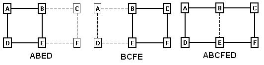
Figure 1A.
If you look at all three loops, you can see that only two loop are necessary to cover all the shots. For example, any of these three combinations cover all the shots:
ABED+BCFE
ABED+ABCFED
BCFE+ABCFED
Now the question becomes, which of these combinations are most useful to cave-surveyors? Thinking through the needs of cave-surveyors, it is fairly easy to define some basic rules for choosing the best loops. Here are the criteria for the best cave-surveying loops:
1. All Shots. The loops must include all the shots in the cave that are part of a loop. In this example, every shots is a part of a loop, so we have to choose loops that cover every shot. At the same time, no one loop covers all the shots, so we have to choose at least two loops. Obviously, if the cave contains shots that aren’t part of a loop, they should be excluded.
2. Smallest Size. The loops should be as “small” as possible. Depending on your needs, “small” could mean the fewest number of shots, the smallest perimeter or the smallest enclosed area. For cave surveyors, choosing loops with the smallest number of shots is probably the best choice. That's because having fewer shots means fewer measurements and that makes it easier to isolate errors. Also, if you have to repair a bad loop in the cave, having fewer shots means less work in the cave.
3. Minimum Overlap. The loops we choose should also have the smallest possible overlap. The reason for this principle is obvious. If lots of loops overlap, errors in one shot can spread over a large number of adjacent shots making it difficult to find the source of the problem. Also, if you are closing loops by distributing errors around a loop, having loops with minimal overlap prevents good loops from being distorted by bad loops.
Going back to Figure 1 above, to satisfy the requirements, we would choose the loops (ABED)+(BCFE), and not (ABED)+(ABCFED) or (BCFE)+(ABCFED) . To clarify why this combination is preferable, look at the follow chart:
|
Loop1 |
Loop2 |
Total Length |
Overlapped Edges |
|
ABED |
BCFE |
8 |
1 |
|
ABED |
ABCFED |
10 |
3 |
|
BCFE |
ABCFED |
10 |
3 |
Figure 2.
As you can see, the combination of the two smaller loops produces the shortest total length and the smallest number of overlapped edges. This pair of loops would be preferable for cave surveyors.
Finding The
Smallest Loops. With simple examples like this one, it is fairly easy to
pick out the best loops. However, as the cave gets bigger with more
interconnected passages, the problem becomes difficult even for a computer
program. This because you have to check every possible combination of
loops to be sure you've got the best ones. That means that the work goes
up exponentially with number of loops and that could make the problem too
time-consuming to be practical for cave survey programs. For example, it might
take a few seconds for small cave, a few hours for a medium sized cave and
months for larger caves.
NP-Complete Problems. This type of problem is described as NP-Complete, [1, 2] which is a mathematical term that describes a situation where the complexity of the goes up exponentially. There is no known method of solving NP-Complete problems in a reasonable amount of time. However, it is often possible to deal with NP-Complete problems by finding a faster solution that does not give mathematically perfect results. In the case of cave surveys, after several months of experimenting, I was able to find a practical solution that gives nearly perfect results and runs relatively fast. To save other surveyors and programmers some time, I will outline the method I used in detail.
Graph Theory. The branch of mathematics that deals with structures like cave-surveys and cave-loops is called “Graph-Theory.” [7] Graph-theory is pretty easy to understand as long as you know the language. For example, in graph-theory, the combination of stations and shots in a cave-survey would be called a “graph.” A station is called a “Vertex” and a shot is called an “Edge.” A loop is called a “Cycle,” and when you find all the cycles in a graph it is called the “Cycle-Basis” for that graph. The following chart that translates the language of cave-surveying to graph-theory:
|
Cave Survey |
Graph Theory |
|
Station |
Vertex |
|
Shot |
Edge |
|
Survey |
Graph |
|
|
Cycle |
|
All Loops |
Cycle Basis |
|
Smallest Loops |
Minimum Cycle Basis |
Using graph-theory nomenclature, to find the best cave-survey loops means we want to find the "Minimum-Cycle-Basis" of the survey-graph.
Spanning-Trees. The first step toward finding loops in a graph or a cave survey is creating something called a “Spanning-Tree.” In a cave-survey language, a spanning-tree would be a series of shots that touches each station in a cave only once. In other words, every station has no more than one shot leading into it. For example, here is a spanning-tree for Figure 1 above:
Figure 2.
As you can see, the spanning-tree touches every station in the cave without visiting any station twice. The shots A-D and B-E have been removed from the survey because, otherwise, stations D and E would have two shots leading into them.
Multiple Spanning-Trees. Another important aspect of spanning-trees is that every graph can have more than one valid spanning-tree. For example, here in another spanning-tree for Figure 1:
Figure 3.
As you can see, this spanning-tree also has one shot leading into each station but it uses a different set of shots to do it.
Finding Loops With Spanning-Trees. The definition of a spanning-tree requires that it not contain any loops (cycles). As a result, any shot that is missing from the spanning-tree, by definition, defines a loop.
For example, in the Figure 3 above, if you put the shot “D – E” back, you will have found the “ABED” loop. In other words, for every shot that is missing from the spanning-tree there is one loop. Thus the “missing shot” is the key to each loop and we will use the missing-shot as a kind of marker for the loops in a cave.
To actually figure out which shots belong to the loop, you follow the “parents” of the missing shots back until they come to a common station. (The arrows in the example graphs show which stations are the parents.) For example, in Figure 3, you follow E back to B and B back to A. This defines one side of the loop. On the other side, you follow D back to A. You stop at A because it is the common parent of both sides loop.
Problems With Spanning-Trees. In the language of Graph-Theory, the loops generated using this approach are called “Fundamental-Cycles.” Unfortunately, fundament-cycles do not satisfy all the criteria that we have set out for cave-surveying. In graph-terminology, what we are looking for is called the “Minimal-Cycle-Basis” of a graph. Although the previous example seems to work perfectly and does find the minimal-cycle-basis, this is not always the case. For example, here is the spanning-tree shown in Figure-2:
Figure 4.
In this case, the missing shots are A-D and B-E. If you look at the loop that is formed when shot A-D is put back into the spanning-tree, you will see it consists of stations A, B, C, D, E, and F. This is the one loop from Figure 1A that we decided was defective.
Different Kinds Of Spanning-Trees. As you can see, the spanning-tree in Figure-3 finds loops that satisfy our cave-survey loop-rules. On the other hand, the the spanning-tree in Figure-4 produces loops that violate thosee rules.
In other words, some kinds of spanning-trees work better than other kinds, and one way to improve loop-quality is to use the right kind of spanning-tree.
Finding Spanning-Trees. To understand how to improve spanning-trees, it is important to understand how they are derived. The process is pretty simple and similar to the way we explore a cave. Generally speaking, you simply “explore” the whole cave and put every shot you find in the spanning-tree unless you have seen the station before. The key to this process is how you “explore.” There are two basic methods of “exploring”: “Depth-First-Search” (DFS) and “Breadth-First-Search” (BFS).
Depth-First-Search. The DFS explores by going to the “back” of the cave first and then works its way back forward. In other words, you don’t linger at each station and you don’t initially explore all branches. Instead, you pick the first connection at each station and follow it deeper. Here is an example of the a DFS spanning-tree for Figure 1:
Figure 5.
In this example we start at A and keep going deeper until we run out of new shots at D. Then we backtrack to E and look for any side branches. There is a side branch running from E to B, but we have already visited B, so we ignore it. This process of backtracking continues until we have checked all side branches and worked our way back to A.
You will notice that this gives the same spanning-tree that we had in Figure 4, which produced the bad, overlapping loops. For the purpose of finding minimum-cycles, a DFS produces poorer loops.
Breadth-First-Search. With BFS, we explore the front of the cave first. We do this by checking all the branches off each station before we move any deeper into the cave. For example, here is a BFS spanning-tree for Figure 1.
Figure 6.
In this example, we start at station A as before, but we explore the connections to B and D before moving on. When we do move on to B, we explore its connections too and continue until we run out of stations that have not been visited. You will notice that this gives the same spanning-tree as Figure 3, which we concluded, gives superior loops. So for our purposes, BFS spanning-trees give superior results.
BFS Problems. Unfortunately, as the loops get more complicated, the BFS trees begin to have problems. For example, here is a more complex survey, the corresponding BFS spanning-tree and the loops it produces:
|
|
|
|
|
More Complex Graph |
BFS Spanning-Tree |
Resulting Loops |
Figure 7.
As you can see, Loop-1 and 2 overlap and Loop-3 and 4 overlap, which is just what we are trying to avoid.
One way to avoid this problem is to change the way we build the spanning-tree. Instead of exploring by depth, we can preferentially choose the stations with most connections to them. In the example above, we would choose E first, because it has four shots connected to it. Next, we would explore B, D, F and H because they have three connections. This is the result:
|
|
|
|
Connections-First BFS Spanning-Tree |
Resulting Loops |
Figure 8.
As you can see, this produces the kind of minimally overlapped loops that we are looking for. (Note: detailed information on implementing these BFS algorithms are available in Manuel Huber’s article [3] in bibliography.)
The Final Problem. Unfortunately, improving the spanning-tree can only be carried so far. Eventually, if you have enough loops, even an optimized spanning-tree fails to produce a minimal-cycle-basis:
|
|
|
Figure 9.
In this example, we have a 3x3 “grid” of loops. As you can see, even using the optimized spanning-tree algorithm, two of the nine loops in the area of F, G, J, K, N and O will be overlapped. Thus, when you have loops stacked three-deep in two directions, even an optimized spanning-tree will generate overlapped loops.
A New Strategy. At this point, we are forced to adopt a new strategy for improving loop quality. We know that a modified BFS spanning-tree will find a set of loops that almost satisfies our criteria, so all we have to do is fix those loops that are sub-optimal. The basic idea is to invent a method to find and fix sub-optimal loops. During my experiments, I found several methods that could be used to do this. The fastest method was to look for “short cuts”.
Looking For Short Cuts. To find short cuts, you look at each loop to see if there is a shorter alternate route. The process begins by selecting one station from the “missing shots” and then doing a Breadth First Search of all adjacent stations. If during the course of the BFS, you find the other end of the “missing shot,” you have a short cut. Since the BFS only explores one “level” of depth at a time, the depth of the search tells you the length of any potential short cut. If the depth exceeds the length of the loop your are trying to improve, you know there is no short cut.
The process is a bit complicated, so here are step-by-step instructions:
1. Choose one loop and note the length of the loop.
2. Choose one station from the “missing shot” for the loop.
3. Do a Breadth First Search of all adjacent shots to this station.
4. Each time you move deeper in the search, keep track of the parent shot.
5. Each time you move deeper, keep track of the depth.
6. If the depth is greater than the length of the loop, there is no short cut for the loop, so you can stop searching.
7. If you encounter the other station in the “missing shot,” you have found a short cut.
8. Create a new loop by collecting all the shots in the short cut. This is done by following the parent shots back to the starting station.
9. Mark the “missing shot” so it is excluded from all futures short-cut searches.
10. Repeat steps 1 through 9 until all loops have been checked for short cuts. You can ignore any loop with less than four shots.
Note: aspects of this algorithm is described in detail in Manuel Huber’s article [3] in bibliography.
Problems With Short Cuts. The “Short Cut” technique works properly for 99% of the loops. However, there are still a few cases where the technique finds sub-optimal loops. This is typical of an NP-Complete problem and we would normally be satisfied with a few sub-optimal loops if the algorithm were fast. In this case, I found a way to improve the technique so it generates nearly 100% minimal loops. (At least in my testing of thousands of random loops, I have yet to find a failure.)
The “Short Cut” technique fails in certain situations where you have two overlapping loops that have the same number of shots. Here is an example:
Figure 10.
On the left, we have a pattern of shots that forms four minimal loops and nine additional, overlapped loops. In some instances, the spanning-tree will find the two overlapping loops shown on the right. (This depends on the order of the shots and how the loops are connected to the rest of the survey.) Since both loops have the same length, the program may choose either loop to process first when it starts to look for short cuts. If the program chooses to process the middle loop first, shots H-E or E-F may be prematurely eliminated from consideration as a short cut. This may cause the program to select overlapped loops around stations {A,B,C,D,E,F}.
Enclosed Area. My solution was to sort the loops by area whenever I found two loops of equal length. This was a bit more complicated to do than it sounds. While it is easy to find the area of an irregular 2D polygon using the “Surveyor’s Rule” or “Determinants”, the surface area of a 3D polygon is difficult to define and calculate. As a result, I chose to find the center of the polygon (centroid), and calculate the average distance to each vertex. This is relatively fast and easy to calculate and gives good results in testing.
Minor Issues. When you combine all the steps outlined above, you have an algorithm that finds minimal loops nearly 100% of the time. In spite of this, there are some situations where the algorithm will find loops that “appear” to be sub-optimal. For example, look at the following diagrams:
Figure 11.
Here you have two possible loops in a graph. Both loops satisfy the requirements of having the minimum number of shots and overlapped edges. However, most people would probably choose the loop on the left as the smallest loop because it has a smaller area. For the purpose of cave surveying, there is no advantage to either loop and both would work just fine. You could add an extra step to the algorithm to fix these cosmetic defects, but it is probably not worth the loss of speed and the extra programming effort.
Running
Time. The running time
for this algorithm is relatively fast.
On a 2.8 Ghz Pentium
4, the test program will find 1,000 loops in a dense grid in 175 milliseconds
and 2,500 loops in about 800 milliseconds. Considering that
Time in milliseconds = M × N × k1+
k2
Where:
M = number of vertices
N = number of edges
k1 = 1.29E-4
k2 = 0.08
Test Software. In order to experiment with different loop finding techniques, I built a test program that is capable of generating and displaying large sets of random and non-random loops. It will find and display minimal loops using this and other algorithms. It will also display various kinds of spanning-trees and you can even save graphs for later analysis. For those who are interested in experimenting with graphs, spanning-trees and minimal cycles, the program can be down loaded here:
https://www.fountainware.com/download/loopfinder.zip
There is no installation program, so you will need to copy the files to a folder and create whatever shortcuts you need. There is a brief help file that explains most of the controls and options. Sources to the main algorithms are included.
Bibliography:
1. Algorithms for generating fundamental cycles
in a graph.
Authors: N. Deo, G. M. Prabhu, and M. S. Krishnamoorthy
ACM Trasn. Math. Software, 8:26-42, 1982.
2. A faster algorithm for Minimum Cycle Basis of
graphs.
Authors: Telikepalli Kavitha, Kurt Mehlhorn, Dimitrios Michail, and Katarzyna Paluch
The 31st International
Colloquium on Automata, Languages and Programming
July 12-16, 2004,
3. Implementation of algorithms for sparse cycle
bases of graphs.
Author: Manuel Huber
4. Implementing Minimum Cycle Basis algorithms.
Authors: Kurt Mehlhorn and Dimitrios Michail
WEA 2005: 4th
International Workshop on
Efficient and
Experimental Algorithms
May 10-13, 2005,
5. Application of Shortest Path Methods.
Author: J.C. de Pina. PhD
thesis,
6. A polynomial-time algorithm to find a shortest
cycle basis of graph.
Author: J. D. Horton.
7.
Graph Theory
Author: Reinhard Diestel
Electronic Edition Available
Here:
http://www.math.uni-hamburg.de/home/diestel/books/graph.theory/index.html