|
|
|
Marching Cubes |
|
Marching Cubes is an algorithm
for converting a 3D surface into a mesh suitable
for computer graphic display. The 3D surface
data can come from a variety of sources.
Isosurfaces. A
common source of surface data is something
called an Isosurface. The prefix
Iso comes from Greek and means
"equal." Thus an Isosurface is a surface that
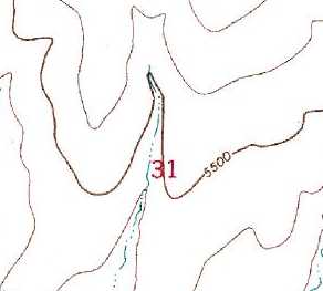
follows points of equal value. As a 2D example, the lines on a weather
map show lines of equal atmospheric
pressure. Likewise, the lines on a
topographic map show lines of equal
elevation. The map to the right shows a
dark-brown line 5,500 that follows
points that are 5,500 feet above sea
level.
|
 |
In the 3D world, the Marching Cube
algorithm allows you to find points of
equal value and, instead of creating a
line, create a surface in the form of a 3D
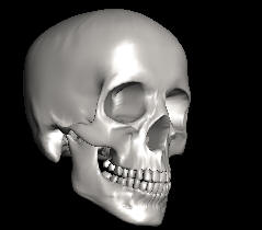
mesh. For example,
you could measure the density of tissue in a
CAT-Scan and create a surface at the point the
tissue becomes hard and dense. Since tissue
become hard and dense at the surface of
a bone, this would allow you to create a 3D
model of a fractured skull to help
surgeons make repairs. The image to the
right shows a human skull reconstructed
from CAT-Scan data using the March Cubes
algorithm.
|
 |
Isosurface Equations. To
illustrate the concept, one way of
creating an isosurface is with a simple
equation. For example, look at the the
equation:
X * X + Y * Y + Z * Z.
It takes an X, Y and Z
argument which are Cartesian Coordinates
for points in 3D space and produces a value for any
point in 3D space. For instance, plugging
the values 1, 2 and 3 into the equation,
you get a value of 14 for that point.
To use the equation to
find a 3D surface, you want to find
points in 3D space where the equation
produces the same value. For example,
here are some example points that
produce values of one. |
 |
|
X |
Y |
Z |
|
Value |
| 1.000 |
0.000 |
0.000 |
= |
1.000 |
| 0.707 |
0.707 |
0.000 |
= |
1.000 |
| 0.707 |
0.000 |
0.707 |
= |
1.000 |
| 0.000 |
0.707 |
0.707 |
= |
1.000 |
| 0.577 |
0.577 |
0.577 |
= |
1.000 |
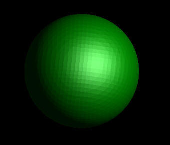
If you examine the
points where the result of the equation
is one, you'll discover they form a
spherical surface. The image to the
above and to the right shows a spherical
surface created with the equation.
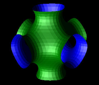
Using a more complex
equation produces a more complex
surface. For example, using the equation
1-(Cos(X)+Cos(Y)+Cos(z)) produces a much
moe complicated surface called a Schwartz
Isosurface. |
 |
|
Generating these meshes is
actually more difficult than it seems. To
find points that are on the surface, you
have to find a large number of points
whose values are all one. This means testing
millions of points, most of which are
nowhere near the surface. The solution
is to use a process called
Marching Cubes.
The Marching Cubes
algorithm simplifies this process by
dividing the 3D space into cubic boxes. The program
only
tests the points at the corners of the
boxes to see if the surface passes
through the box. If the surface passes
through box, the exactly location of the
surface is calculated by
interpolation. |
 |
For example, using the sphere
equation we can calculate
where the surface of the sphere intersects the
cube. In example to the
right,
the black numbers represent the corner
coordinates of the one side of the cube.
The red numbers show the
sphere-equation value for those
coordinates. As you can see, the surface
of the sphere, (as represented by the
1-value,) falls somewhere along the top
and right sides of the box. By
interpolating, we can find the exact
location. |
 |
|
Since the ultimate goal
is to create a 3D mesh, we have to find
the places where the surface intersects
each cubes and create triangles that
correspond to the planes of
intersections. Since there are only a
limited number of ways these
planes of intersections can occur, we
can rapidly determine where the
triangles need to be placed. Once we
where the triangles need to places we
can determine the exact location
interpolating the intersection points
just like we did with the 2D example
above.
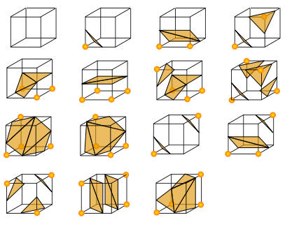
The Drawings to
the right show all the possible
combinations. Corners with an orange dot
are inside the surface. Points without a
dot are outside. |
|
|
The triangles shown are
based on the pattern of dots that are
inside and outside the surface. For more
details on the Marching Cubes algorithm,
click here. |
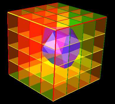
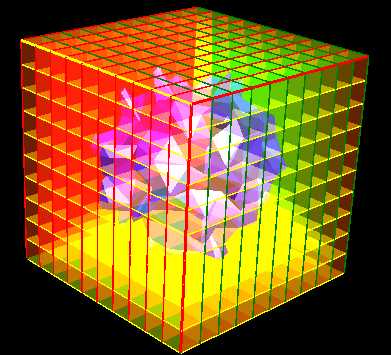
Resolution. The resolution of the
mesh generated by the Marching Cubes algorithm
is controlled by the number of cubes. The more
cubes, the smaller each cube and the more detail
the algorithm captures.
On the other hand, the number of cells goes up
by the cube of the number of grid lines. That
means a 5 x 5 x 5 grid will have 125 cells, a 10
x 10 x 10 grid will have 1,000 cells and a 100
x 100 x 100 cell
grid will have 1 million cells.
As a result, the processing time also goes up by
the number cube of the grid lines. For example,
a 50 x 50 x 50 grid can be process in one
second, 100 x 100 x 100 takes 5 seconds
and a 200 x 200 x 200 takes 36 seconds. |
 |
|
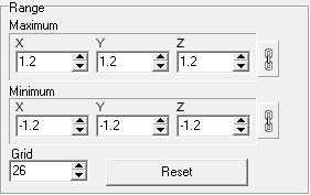
To control the resolution,
Mandelbrot 3D allows you to set the number of
grid lines. The "Grid" option shown to the right
sets the number of grid lines.
Range. The Maximum and
Minimum range values are the 3D coordinates of
the minimum and maximum range covered by the
Marching Cubes algorithm. Setting the smaller
values allows you to focus on smaller portions
of the surface. |
 |
|
|
|
|
|
|